Mathematics & Education · Calculus
Calculus Formula Chart for Limits, Derivatives and Integrals
Use the chart to review limit laws, derivative rules, common antiderivatives, definite-integral formulas, integration techniques, convergence tests, and Taylor expansions with their required conditions.
A formula is valid only under its hypotheses. Check the function domain, continuity, differentiability, denominator restrictions, interval orientation, and convergence conditions before using a result.
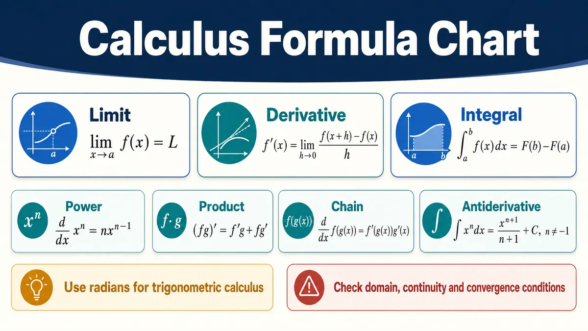
Quick answer
Calculus connects approach, change and accumulation
Limits describe approach. Derivatives use limits to measure instantaneous change. Integrals accumulate quantities and reverse differentiation through the Fundamental Theorem. Infinite series extend these ideas by representing sums and functions with infinitely many terms.
The formulas below align with the scope of the peer-reviewed OpenStax Calculus Volume 1, which covers limits, derivatives, integration, and their applications.
Foundation
Limits
Limits describe approach and make derivative and integral definitions precise.
Instantaneous change
Derivatives
A derivative gives tangent slope and instantaneous rate where it exists.
Accumulation
Integrals
A definite integral measures signed accumulation across an interval.
Infinite processes
Series
Convergence tests determine whether infinitely many terms approach a finite sum.
Calculus concepts at a glance
These concise answers summarize the most frequently used distinctions and conditions. Use the detailed tables for formulas and exceptions.
What does a limit describe?
A limit describes the value a function approaches as its input approaches a point.
What does a derivative measure?
A derivative measures instantaneous rate of change and tangent-line slope.
What does a definite integral measure?
A definite integral measures signed accumulation over an interval.
When does direct substitution work?
Direct substitution works when the function is continuous at the target and the substituted value stays in its domain.
What is the derivative of x^n?
The derivative of x^n is nx^(n−1) wherever the real power rule applies.
When is the chain rule required?
Use the chain rule when one differentiable function is nested inside another.
Why does an indefinite integral include C?
The constant C represents all antiderivatives that differ only by a constant.
How do you evaluate a definite integral?
Find an antiderivative F and calculate F(b)−F(a) when the Fundamental Theorem applies.
When does a geometric series converge?
A geometric series converges when the absolute value of its common ratio is less than 1.
Does a_n approaching zero prove convergence?
No. Terms approaching zero are necessary for series convergence but are not sufficient.
What is a Taylor polynomial?
A Taylor polynomial uses finitely many derivative terms to approximate a function near a chosen center.
Should calculus trigonometry use degrees?
Standard calculus derivative and integral formulas use radians, not degrees.
See how the major calculus ideas connect
Limits define derivatives and integrals. Derivatives describe change, integrals reconstruct accumulated change, and series build functions from infinitely many terms.
Step 1
Limits
x → a
Describe approach, continuity, and indeterminate forms.
Step 2
Derivatives
f′(x)
Measure instantaneous rate, slope, optimization, and local behavior.
Step 3
Integrals
∫ f(x)dx
Measure accumulation, net change, area, volume, and average value.
Step 4
Series
Σ aₙ
Represent infinite sums and approximate functions with power series.
Limit Laws and Continuity Conditions
Use these laws when the component limits exist and every stated condition is satisfied. Direct substitution works whenever the function is continuous at the point.
Swipe horizontally inside the table to view every column.
| Rule | Formula | Conditions | Meaning |
|---|---|---|---|
| Constant law | lim x→a c = c | c is constant | A constant keeps the same value. |
| Identity law | lim x→a x = a | None | The input approaches the target value. |
| Sum and difference | lim(f ± g) = L ± M | lim f = L and lim g = M | Take limits term by term. |
| Constant multiple | lim(cf) = cL | c is constant and lim f = L | A constant factor passes through the limit. |
| Product law | lim(fg) = LM | Both component limits exist | Multiply the component limits. |
| Quotient law | lim(f/g) = L/M | M ≠ 0 — Nonzero denominator condition | Divide the limits only when the denominator limit is nonzero. |
| Power law | lim[f(x)]^n = L^n | n is a positive integer | Apply the power after taking the limit. |
| Root law | lim ⁿ√f(x) = ⁿ√L | For even n, require L ≥ 0 in real calculus | Roots pass through limits on their valid domain. |
| Composition | lim h(f(x)) = h(L) | h is continuous at L | Evaluate the outer continuous function at the inner limit. |
| Continuity test | lim x→a f(x) = f(a) — Definition of continuity at a point | f(a) exists and the two-sided limit exists | A continuous function has no break at a. |
| Squeeze theorem | g ≤ f ≤ h and lim g = lim h = L ⇒ lim f = L | Inequalities hold near a | Matching outer limits force the middle limit. |
L and M denote finite limits unless a row states otherwise.
- • A two-sided limit exists only when the left-hand and right-hand limits agree.
- • An expression such as 0/0 is indeterminate; it signals that more work is needed, not that the limit equals zero.
- • Check the function domain before applying direct substitution, roots, logarithms, or quotient rules.
Download or export
How to evaluate an unfamiliar limit
- 1. Substitute first. A finite value often finishes the problem immediately.
- 2. Classify the obstacle. Check for 0/0, nonzero/0, infinity behavior, oscillation, or domain failure.
- 3. Transform carefully. Factor, rationalize, combine fractions, use identities, or apply an eligible theorem.
- 4. Verify both sides. A two-sided limit requires matching one-sided limits.
Core Derivative Rules
Derivative rules calculate instantaneous rates of change. Keep the original function structure visible before choosing a rule.
Swipe horizontally inside the table to view every column.
| Rule | Formula | When to use it | Example |
|---|---|---|---|
| Definition | f′(a) = lim h→0 [f(a+h)−f(a)]/h | To define or derive a derivative from first principles | For f(x)=x², f′(a)=2a |
| Constant rule | d/dx[c] = 0 | A term has no x-dependence | d/dx[7] = 0 |
| Power rule | d/dx[x^n] = nx^(n−1) | Real powers where the expression is defined | d/dx[x⁵] = 5x⁴ |
| Constant multiple | d/dx[cf] = cf′ | A constant multiplies a function | d/dx[4sin x] = 4cos x |
| Sum and difference | d/dx[f ± g] = f′ ± g′ | Terms are added or subtracted | d/dx[x³−2x] = 3x²−2 |
| Product rule | (fg)′ = f′g + fg′ — Product rule | Two variable functions are multiplied | d/dx[x²e^x] = 2xe^x + x²e^x |
| Quotient rule | (f/g)′ = (f′g−fg′)/g² | One function is divided by another | d/dx[x/sin x] = (sin x−x cos x)/sin²x |
| Chain rule | d/dx[f(g(x))] = f′(g(x))g′(x) — Chain rule | One function is composed inside another | d/dx[(3x+1)⁵] = 15(3x+1)⁴ |
| Implicit differentiation | Differentiate both sides with respect to x | x and y are linked by an equation | x²+y²=1 ⇒ y′=−x/y |
| Inverse-function rule | (f⁻¹)′(x) = 1/f′(f⁻¹(x)) | Differentiate an inverse where f′ is nonzero | d/dx[ln x] = 1/x |
Angles in trigonometric derivative formulas use radians.
- • The product derivative is not f′g′, and the quotient derivative is not f′/g′.
- • For the chain rule, multiply by the derivative of every nested inner function.
- • A derivative may fail to exist at corners, cusps, vertical tangents, or discontinuities.
Download or export
Common Function Derivatives
These formulas assume the input lies in the real domain of the function. Apply the chain rule when x is replaced by an inner function u(x).
Swipe horizontally inside the table to view every column.
| Function f(x) | Derivative f′(x) | Domain or condition | Chain-rule form |
|---|---|---|---|
| x^n | nx^(n−1) | Where the real power is defined | d/dx[u^n] = nu^(n−1)u′ |
| e^x | e^x | All real x | d/dx[e^u] = e^u u′ |
| a^x | a^x ln a | a > 0 and a ≠ 1 | d/dx[a^u] = a^u ln(a)u′ |
| ln x | 1/x | x > 0 — Natural logarithm domain | d/dx[ln|u|] = u′/u for u ≠ 0 |
| log_a x | 1/(x ln a) | x > 0, a > 0, a ≠ 1 | d/dx[log_a u] = u′/(u ln a) |
| sin x | cos x — Sine derivative | x in radians | d/dx[sin u] = cos(u)u′ |
| cos x | −sin x | x in radians | d/dx[cos u] = −sin(u)u′ |
| tan x | sec²x | cos x ≠ 0 | d/dx[tan u] = sec²(u)u′ |
| sec x | sec x tan x | cos x ≠ 0 | d/dx[sec u] = sec(u)tan(u)u′ |
| arcsin x | 1/√(1−x²) | |x| < 1 | d/dx[arcsin u] = u′/√(1−u²) |
| arctan x | 1/(1+x²) | All real x | d/dx[arctan u] = u′/(1+u²) |
| sinh x | cosh x | All real x | d/dx[sinh u] = cosh(u)u′ |
Use radians for trigonometric functions in standard calculus formulas.
- • The formula d/dx[ln|u|] = u′/u works on intervals where u does not cross zero.
- • Inverse-trigonometric derivative domains must be checked before substituting values.
- • A table entry gives a local rule; it does not remove the need to simplify or state excluded values.
Download or export
Browser-only educational tool
Polynomial derivative and definite-integral calculator
Enter coefficients for f(x)=ax³+bx²+cx+d. The tool differentiates the polynomial, evaluates f and f′ at one input, and applies the Fundamental Theorem to a definite integral. Inputs stay in the browser.
Polynomial
f(x) = x³ −2x² +3x +1
- Derivative formula
- f′(x) = 3x² −4x +3
- Function at x=2
- 7
- Derivative at x=2
- 7
- Antiderivative family
- F(x) = 0.25x⁴ −0.66666667x³ +1.5x² +x + C
- F(2)
- 6.66666667
- F(0)
- 0
- Integral from 0 to 2
- 6.66666667
- Evaluation step
- F(2) − F(0)
The definite integral is signed accumulation. It is not automatically geometric area when the polynomial crosses the x-axis inside the interval.
Basic Antiderivatives and Integrals
An indefinite integral represents a family of antiderivatives, so include the constant C. Definite integrals return a number and do not take an added C.
Swipe horizontally inside the table to view every column.
| Integrand | Antiderivative | Condition | Useful recognition |
|---|---|---|---|
| x^n | x^(n+1)/(n+1) + C | n ≠ −1 — Power rule excludes exponent negative one | Increase the exponent by 1, then divide. |
| 1/x | ln|x| + C — Natural logarithm antiderivative | x ≠ 0 | The power rule cannot use n = −1. |
| e^x | e^x + C | All real x | Exponential base e is unchanged. |
| a^x | a^x/ln a + C | a > 0 and a ≠ 1 | Divide by ln a. |
| sin x | −cos x + C | x in radians | Differentiate −cos x to check. |
| cos x | sin x + C | x in radians | Differentiate sin x to check. |
| sec²x | tan x + C | cos x ≠ 0 | Recognize a tangent derivative. |
| sec x tan x | sec x + C | cos x ≠ 0 | Recognize a secant derivative. |
| 1/(1+x²) | arctan x + C | All real x | Inverse-tangent pattern. |
| 1/√(1−x²) | arcsin x + C | |x| < 1 for the integrand | Inverse-sine pattern. |
| f′(x)/f(x) | ln|f(x)| + C | f(x) ≠ 0 | Logarithmic substitution pattern. |
| f′(x)e^(f(x)) | e^(f(x)) + C | Where f is differentiable | Reverse chain-rule pattern. |
C is an arbitrary real constant on each interval of the domain.
- • Always differentiate an antiderivative to verify it reproduces the integrand.
- • Absolute value is required in ln|x| and ln|f(x)| when the input may be negative.
- • Indefinite-integral formulas can change form across disconnected domain intervals.
Download or export
Definite Integrals and Fundamental Theorem Formulas
Definite integrals measure signed accumulation. The Fundamental Theorem connects accumulation with antiderivatives.
Swipe horizontally inside the table to view every column.
| Concept | Formula | Conditions | Interpretation |
|---|---|---|---|
| Riemann-sum definition | ∫_a^b f(x)dx = lim n→∞ Σ f(x_i*)Δx | The limit exists | Adds increasingly narrow rectangle contributions. |
| Fundamental Theorem, evaluation | ∫_a^b f(x)dx = F(b)−F(a) — Fundamental Theorem evaluation formula | F′=f and f is integrable | Evaluate any antiderivative at the bounds. |
| Fundamental Theorem, accumulation | d/dx ∫_a^x f(t)dt = f(x) | f is continuous near x | Differentiation reverses accumulation. |
| Reversed bounds | ∫_b^a f(x)dx = −∫_a^b f(x)dx | Integral exists | Reversing direction changes the sign. |
| Additivity | ∫_a^b f + ∫_b^c f = ∫_a^c f | All integrals exist | Split or join adjacent intervals. |
| Average value | f_avg = [1/(b−a)]∫_a^b f(x)dx | a < b and f is integrable | Mean function value over an interval. |
| Net change | F(b)−F(a) = ∫_a^b F′(x)dx | F is differentiable and F′ integrable | Accumulated rate equals total change. |
| Area between curves | A = ∫_a^b [top(x)−bottom(x)]dx | Top stays above bottom — Ordering condition for area formula | Geometric area between two graphs. |
| Washer volume | V = π∫_a^b [R(x)²−r(x)²]dx | Cross-sections are washers | Volume of revolution around an axis. |
| Arc length | L = ∫_a^b √(1+[f′(x)]²)dx | f′ is continuous | Length of a smooth graph segment. |
The variable of integration is a dummy variable; use a different symbol inside accumulation functions when helpful.
- • A definite integral is signed area; geometric area requires splitting where the function changes sign or using absolute value appropriately.
- • The Fundamental Theorem requires an antiderivative and the stated regularity conditions.
- • Application formulas must match the geometry, axis, and units of the problem.
Download or export
Integration Techniques and Selection Clues
Choose a technique by recognizing structure. Algebraic simplification often reveals a basic antiderivative before a more advanced method is needed.
Swipe horizontally inside the table to view every column.
| Technique | Core formula or action | Best clue | Typical example |
|---|---|---|---|
| u-substitution | Let u=g(x), du=g′(x)dx | An inner function appears with its derivative — Substitution clue | ∫2x cos(x²)dx |
| Integration by parts | ∫u dv = uv − ∫v du | A product becomes simpler after differentiating one factor | ∫x e^x dx |
| Trigonometric identities | Rewrite using identities before integrating | Powers or products of trig functions | ∫sin²x dx |
| Trigonometric substitution | Use x=a sin θ, a tan θ, or a sec θ | Radicals contain a²−x², a²+x², or x²−a² | ∫dx/√(a²−x²) |
| Partial fractions | Decompose a rational function | Proper rational function with factorable denominator | ∫dx/(x²−1) |
| Complete the square | Rewrite a quadratic into shifted-square form | Irreducible quadratic or inverse-trig pattern | ∫dx/(x²+4x+8) |
| Improper integral | Replace an infinite bound or discontinuity with a limit | Infinite interval or unbounded integrand — Improper integral condition | ∫_1^∞ 1/x² dx |
| Numerical integration | Approximate with rectangles, trapezoids, or Simpson-type rules | No elementary antiderivative or only sampled data | Estimate ∫_0^1 e^(−x²)dx |
Technique choice does not replace domain checks, convergence checks, or verification by differentiation.
- • Simplify algebraically and factor constants before selecting a technique.
- • Improper integrals converge only when the defining limit exists and is finite.
- • A numerical estimate should state the method, interval, subinterval count, and error tolerance when known.
Download or export
Choose an integration method by structure
Start by simplifying the integrand. Use substitution for a reverse chain-rule pattern, integration by parts for a product that becomes simpler, partial fractions for suitable rational functions, and a limit definition for improper integrals. Differentiate the final antiderivative to check it.
Sequences, Series and Convergence Tests
A series is the limit of its partial sums. Passing one test proves only what that test guarantees, so verify every hypothesis.
Swipe horizontally inside the table to view every column.
| Pattern or test | Criterion | Conclusion | Important limitation |
|---|---|---|---|
| Geometric series | Σ ar^n from n=0 converges when |r|<1 | Sum = a/(1−r) | Diverges when |r|≥1 |
| p-series | Σ 1/n^p | Converges for p>1; diverges for p≤1 | Applies to this exact power pattern |
| Divergence test | If lim a_n ≠ 0 or does not exist | Σa_n diverges | If lim a_n=0, the test is inconclusive — Divergence test limitation |
| Integral test | a_n=f(n), with f positive, continuous, decreasing | Σa_n and ∫f have the same convergence behavior | All three hypotheses matter |
| Direct comparison | 0≤a_n≤b_n eventually | Use a known larger convergent or smaller divergent series | Direction of comparison is crucial |
| Limit comparison | lim a_n/b_n = L with 0<L<∞ | The positive-term series behave alike | Requires a finite positive comparison limit |
| Ratio test | L=lim |a_(n+1)/a_n| | Converges if L<1; diverges if L>1 | Inconclusive when L=1 |
| Root test | L=lim ⁿ√|a_n| | Converges if L<1; diverges if L>1 | Inconclusive when L=1 |
| Alternating-series test | b_n decreases to 0 | Σ(−1)^n b_n converges | May converge conditionally rather than absolutely |
| Absolute convergence | Σ|a_n| converges | Σa_n converges | The converse is false |
| Power-series interval | Test endpoints separately after finding radius R | Converges inside |x−c|<R | Endpoint behavior is not determined by R alone — Endpoint testing required |
Series notation assumes the stated starting index; changing the index can change the first term but not convergence behavior after finitely many terms.
- • A necessary condition for Σa_n to converge is a_n→0, but that condition alone is not sufficient.
- • Absolute convergence implies convergence; conditional convergence does not imply absolute convergence.
- • For a power series, always test each endpoint separately after finding the radius of convergence.
Download or export
Taylor and Maclaurin Series Formulas
A Taylor series represents a function near a center when the series converges to that function. Maclaurin series use center c=0.
Swipe horizontally inside the table to view every column.
| Function or formula | Series about 0 | Interval or domain note | First terms |
|---|---|---|---|
| General Taylor series | Σ f^(n)(c)(x−c)^n/n! | Convergence to f must be established — Convergence to function must be proved | f(c)+f′(c)(x−c)+f″(c)(x−c)²/2!+… |
| e^x | Σ x^n/n! — Exponential Maclaurin series | All real x | 1+x+x²/2!+x³/3!+… |
| sin x | Σ (−1)^n x^(2n+1)/(2n+1)! | All real x | x−x³/3!+x⁵/5!−… |
| cos x | Σ (−1)^n x^(2n)/(2n)! | All real x | 1−x²/2!+x⁴/4!−… |
| 1/(1−x) | Σ x^n | |x|<1 | 1+x+x²+x³+… |
| ln(1+x) | Σ (−1)^(n+1)x^n/n, n≥1 | −1<x≤1 with endpoint behavior checked | x−x²/2+x³/3−… |
| arctan x | Σ (−1)^n x^(2n+1)/(2n+1) | |x|≤1 with endpoint behavior checked | x−x³/3+x⁵/5−… |
| Binomial series | (1+x)^α = Σ C(α,n)x^n | |x|<1 in the general noninteger case | 1+αx+α(α−1)x²/2!+… |
| Taylor remainder bound | |R_n(x)| ≤ M|x−c|^(n+1)/(n+1)! | |f^(n+1)|≤M between c and x | Bounds truncation error. |
Factorial n! means n(n−1)…2·1, with 0!=1.
- • A Taylor polynomial is finite; a Taylor series contains infinitely many terms.
- • Matching derivatives at the center does not by itself prove that the infinite series equals the function away from the center.
- • State the center and interval of convergence whenever a power series is used.
Download or export
Interpret calculus results with units and context
Derivative units
If f measures distance in meters and x measures time in seconds, f′ has units of meters per second. A second derivative then has meters per second squared.
Integral units
Integrating a rate multiplies its output unit by the input unit. Integrating meters per second with respect to seconds produces meters.
Signs matter
A negative derivative means the function is decreasing locally. A negative definite integral means negative signed accumulation, not negative geometric area.
Approximation has error
Numerical integration and truncated Taylor polynomials are approximations. State the interval, method, number of terms or subintervals, and an error estimate when available.
Common calculus mistakes to avoid
Ignoring hypotheses
Do not apply a theorem before checking continuity, differentiability, denominator, domain, or convergence conditions.
Dropping the inner derivative
The chain rule requires multiplication by the derivative of every nested inner function.
Using the product rule incorrectly
The derivative of fg is f′g+fg′, not f′g′.
Forgetting the constant
Include +C for indefinite integrals, but not after evaluating a definite integral.
Treating signed area as total area
Split the interval at zeros or integrate an absolute value when geometric area is required.
Concluding from a_n→0
A zero term limit does not prove that a series converges. The harmonic series is a standard counterexample.
Skipping endpoint tests
A power-series radius does not decide convergence at either endpoint. Test both separately.
Using degrees in derivative formulas
Standard trigonometric calculus formulas assume radians.
Frequently asked questions
What are the main branches of single-variable calculus?
Differential calculus studies instantaneous change, while integral calculus studies accumulation. Limits support both branches and make their definitions precise.
What is a limit?
A limit describes the value a function approaches as the input approaches a point. The function does not always need to equal that value at the point.
When can you use direct substitution for a limit?
Use direct substitution when the function is continuous at the target input and the substituted expression stays in its domain.
What does a derivative measure?
A derivative measures instantaneous rate of change. Geometrically, it gives the slope of the tangent line where that slope exists.
What is the derivative of x to the n power?
The derivative of x^n is nx^(n−1) wherever the real power rule applies.
When should you use the chain rule?
Use the chain rule when one differentiable function is nested inside another. Differentiate the outer function and multiply by the derivative of the inner function.
What is an antiderivative?
An antiderivative of f is a function F whose derivative equals f. Indefinite integrals represent families of antiderivatives.
Why does an indefinite integral need plus C?
Functions that differ by a constant have the same derivative. The constant C represents every member of the antiderivative family.
What does a definite integral measure?
A definite integral measures signed accumulation over an interval. In a graph, it equals area above the axis minus area below the axis.
What does the Fundamental Theorem of Calculus say?
The theorem connects differentiation and integration. It lets you evaluate a definite integral with an antiderivative and differentiates accumulation functions under suitable conditions.
When should you use u-substitution?
Use u-substitution when the integrand contains an inner function together with a constant multiple of its derivative.
What is an improper integral?
An improper integral has an infinite interval or an unbounded integrand. It converges only when its defining limit exists and is finite.
What condition must every convergent series satisfy?
Its terms must approach zero. Terms approaching zero are necessary for convergence but do not prove convergence by themselves.
When does a geometric series converge?
A geometric series with ratio r converges when |r| is less than 1. Its sum is the first term divided by 1−r.
What is the difference between a Taylor polynomial and a Taylor series?
A Taylor polynomial uses finitely many derivative terms. A Taylor series is the infinite limit of those terms when the series converges.
Should trigonometric calculus formulas use degrees or radians?
Standard derivative and integral formulas use radians. Degree input introduces additional conversion factors.
Sources
OpenStax, Rice University — Calculus Volume 1
Peer-reviewed reference for limits, derivative definitions and rules, applications of derivatives, integration, and the Fundamental Theorem of Calculus.
https://openstax.org/details/books/calculus-volume-1
OpenStax, Rice University — Calculus Volume 2
Peer-reviewed reference for integration techniques, differential equations, sequences, series, and power series.
https://openstax.org/details/books/calculus-volume-2
National Institute of Standards and Technology — Digital Library of Mathematical Functions
Authoritative reference for standard notation, elementary-function derivatives, integrals, and series expansions.
https://dlmf.nist.gov/